Urban Transportation & Logisitics Systems

Introduction

09/08/2020

Itenyu - urban transportation student group

Course is focused on mathmatcial modelling regarding logistics problems such as congestion, or the space-time element.

Red Hook largest electric fleet

• how do you decided how many stations?

Professor Chow: joseph.chow@nyu.edu TA: Chloe bl2453@nyu.edu - office hour 2 - 4 pm Tuesdays

"Logisitics may be defined as the design and operation of the physical, managerial, and information systems neeeded to allow goods to overcome time and space" - Daskin, 1985

Density has explicity effects on performance --> congestion spatial and temporal heterogeneity

Course Objectives

1. determine the most appropriate opimization methods to apply to an urban logistics problem
2. Design and evaluate transportat systems and their operational strategies using optimization models and algorithims.

Grades

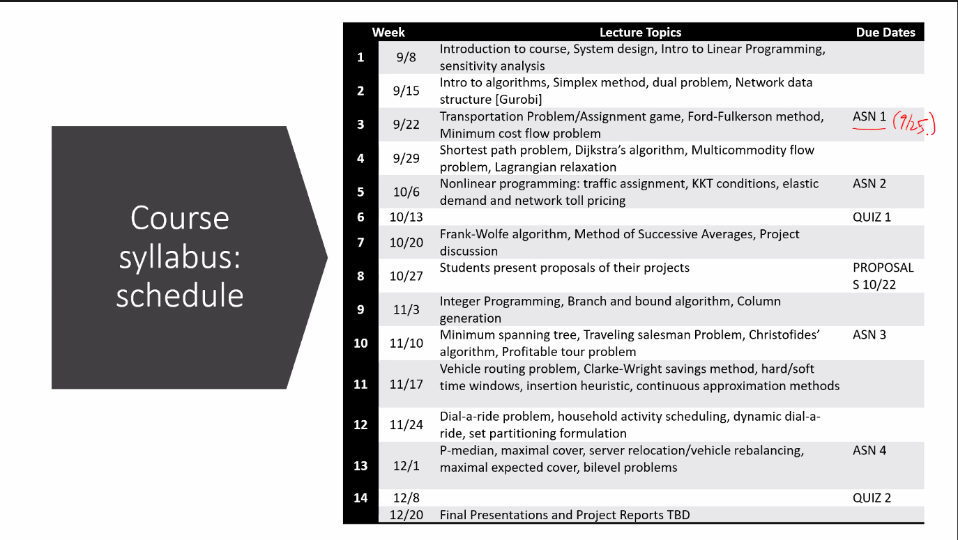
4 assignments 40% 2 Quizzes 30% ( 15% each ) Project 30%

Quizzes are true/false with justification - TEST YOUR MIGHT!!

References

• https://trid.trb.org
• https://scholar.google.com

Definitions

• Deterministic - all variables fed into the model are static within a given range.
• Stochastic - introducing randomness into the variables.

;

Thinking about how to model Bimodel transportation

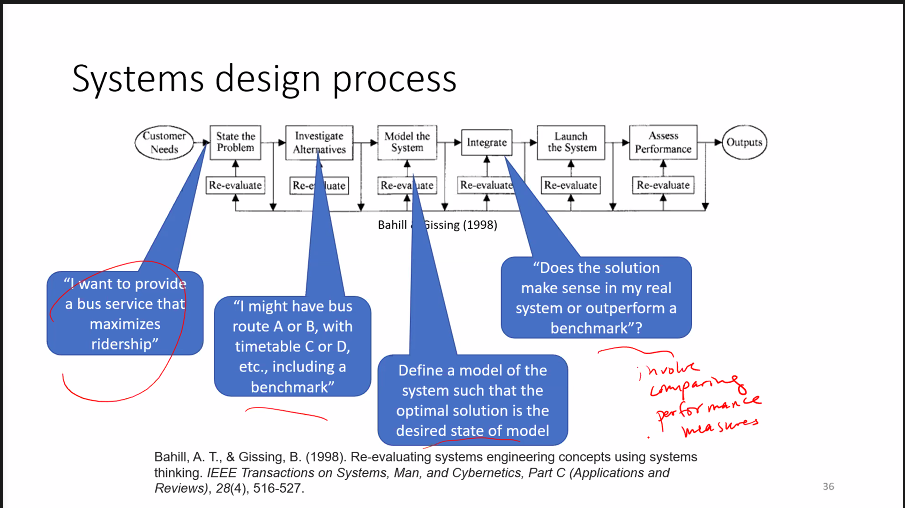
Identifying performance metrics by setting a benchmark to compare.

• define a model
• set a solution
• compare solution to benchamrk

bimodal ride share - having or involving two modes, in particular (of a statistical distribution) having two maxima.

Parameterize the travel demand to back out how many people possibly on average require last mile transportation in the given area. Attempt to figure out how much of this population is being serviced by the current transportaiton, and subtract out what population requires additional transportation.

optimize for vehicle occupancny by looking at different parameters like

• land use
• zoning
• travel demand
• trip demand
• static or dynamic pickup locations

Spatial/temporal element!!

Quesitons based on the optimization

How do you match people to vehicles? How long is each trip? Measure comfort?

Modelling

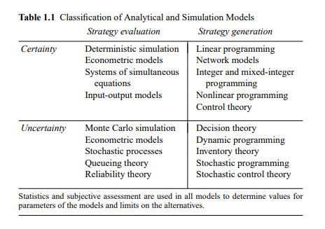
We are looking to describe a system such that the optimal solution satisfies our desired design

• trade-off analysis can then be made to understand real life impacts of decisions.

Model: a mathematical relationship between variables

• descriptive model - used to mimic reality
• normative model - used to define desired design
  • optimization model - relating variables under an optimial condition

Algorithm: a set of instructions to perform on variables.

• for optimization models algorithms needed to determine the variables under optimal condition.

Operational policy: a rule employed by a decision-maker or policy-maker ( basically many of our products are operational policies )

Mathematical Programming ( MP )

;

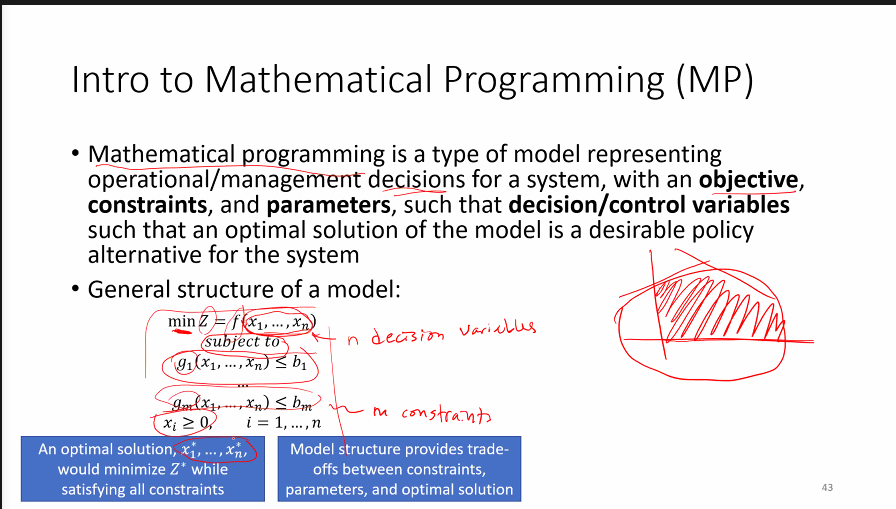
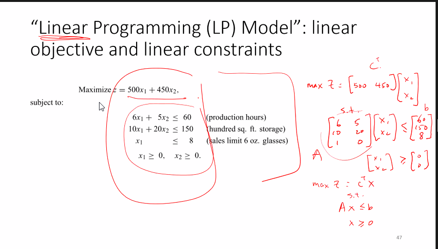
Mathematical programming is a type of model representing operational/management decisions for a system, with an objective, constraints, and parameters, such that decision/controls variables such that an optimal solution of the model is a desirable policy.

How do a i chose a value of x that satisfies the equation? Where x is a set of n number of variables can be a number of constraints.

An optimal solution x1 ... xn would minimize desired variable Z while satisfying all constraints.

Example

Lemma 1.4 Any solution to a linear programming problem that is a local minimum solution is also the global minimum solution.

Note: a solution is not guaranteed to be unique, and a model may not even have an optimal solution

Example

George Dantig

Reading

Chapter 1

link

;

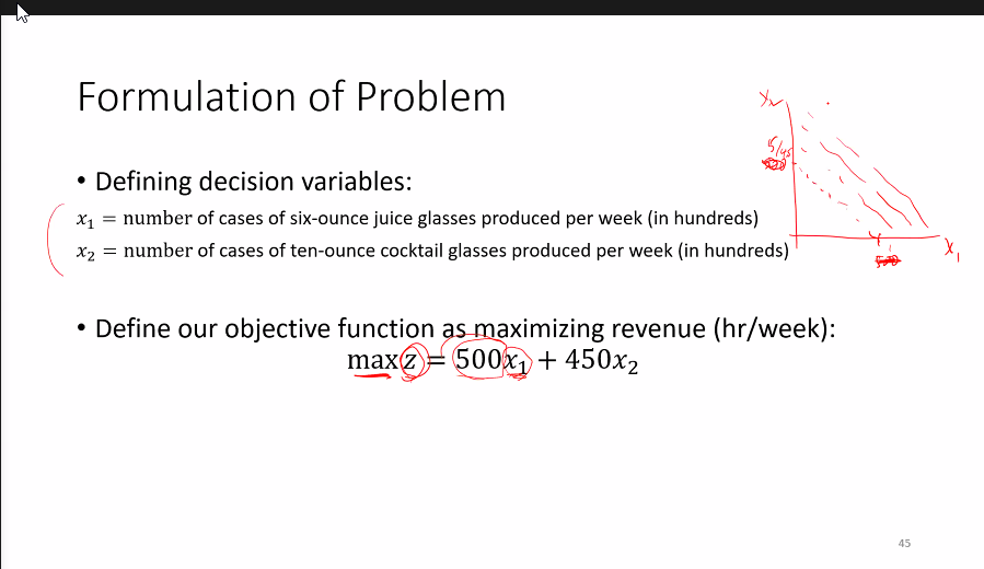
objective function - criterion the decision maker will use to evaluate alternative solutions to the problem.

Chapter 2 Simplex Method

The simplex method can solve any linear program!

---

Simplex Algorithm, sensitivity analysis and duality.

09/15/2020

practice graphical

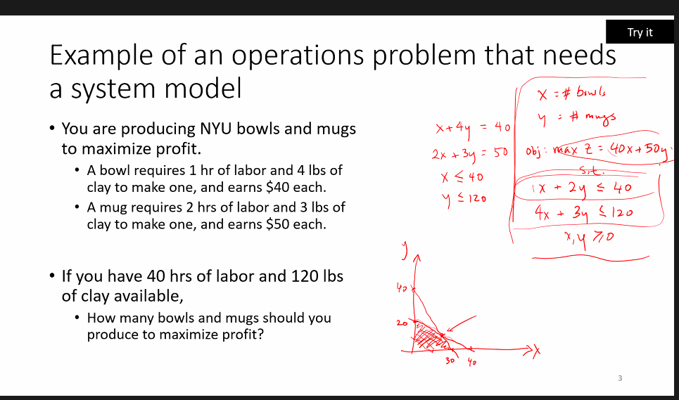
function in excel called solver uses an algorithm called simplex.

file ---> options --> addins --> solver addin tool -- > data --> solver

use simplex LP

Readings

BHM77 Ch 2 -4 Ahuja et al - Network Flows CH 3 ( on classes ) Samuelson P. A. Spatial price equilibrium and linear programming. The American economic review

Samuelson first american to win nobel prize

slack variable equals 0, implies constraint is binding.

when choosing a entry point, you chose the variable with the most impact to the objective equation.

How to transform min/max into Duel problem

Solve simplex method maximization problem

solve linear program graphically

canonical form

1. non-negative
2. all constraints are in equality
3. right-hand coefficients are all non-negative
4. one decision variable is isolated in each constraint ( in the basis ) there should be m basic variables at any iteration.

turning a minimizing problem to a maximize by multiplying everything by -1

transform inequality function by adding a slack variable.

Shadow Price - how much the value of an objective (optimal) function changes due to a marginal variation in the right-hand side of a constraint. It is assumed that the rest of the model’s parameters remain constant.

duel problems is A -t ( A transpose ).

Homework 1.

Resources

running model in excel

Question 2a. How do you get ton-miles?

Question 3.

Readings

• BHM77 Chapter 8

Objectives

• Represent Systems as networks using different data structures

• Differentiate between a transportation problem and a minimum cost flow problem

• interpreting the results of optimal solutions to the problems.

Terms

shadow price - one shadow price per constraint, whereas each constraint increases by 1 unit.

network - graph containing a set of nodes and a set of links G(N)(A)

c _a - cost of traversing link a.

q ^rs - demand between node r and node s

x a - is flow on link a

K - set of paths

Notes

Node Link model will have m(n-2) number of zeros. Not very efficient for computational models.

Node Adjacency matrix - used for social networks

link list - ( basically a csv )

Sioux Falls - popular benchmark marker ( larry leBlanc )

if flow is less than capacity - shadow price is 0

Shortest path problem and multicommodity flow

09/29/2020

Objectives

• shortest path problem (SPP) as a special case of minimum cost flow problem
  • Dijkstra's algorithm to solve SPP
• Successive shortest path algorithm to solve minimum cost flow problem
• decomposition approach is based on
  • Lagrangian relaxation.

Readings

BHM77 Ch 8, Ch 12 Tutorial for Dijkstra Ahuja 1993 Ch 9.7

Strong Duality

if shadow prices is equal to 0, then it is binding, if greater than 0, the binding.


Dijkstra's label setting algorithm

1. All notes besides origin s are labeled open.
2. update distances w and predecessors p of nodes immediately downstream from last closed node i
3. select open node i with smallest w add to closed set
4. repeat 1 and 2 until desired destination is closed.

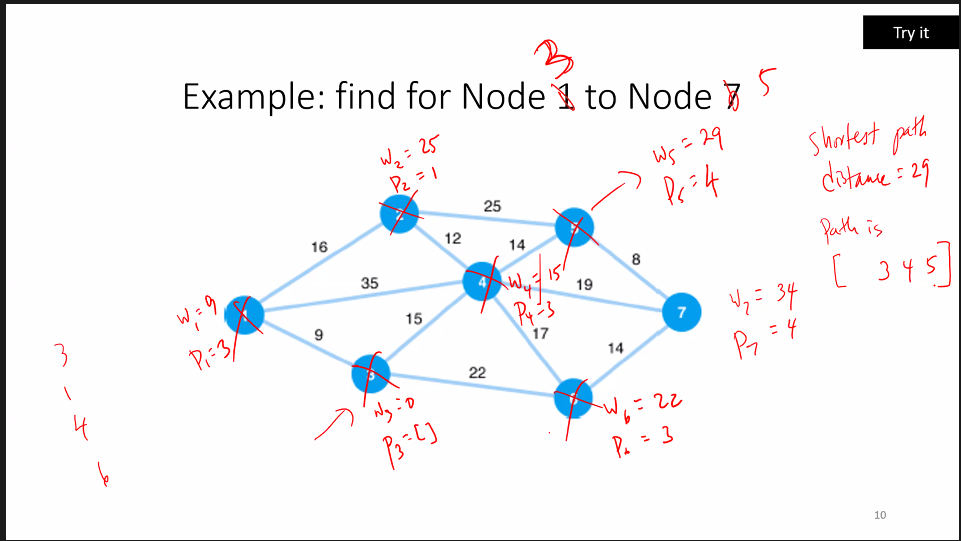
label setting - every iteration of the algorithm we say whether it is open or closed.

1:1 algorthim will stop when the destination node is closed. This is because each iteration a node closes, a node closes when it can o longer be changed.

w = distance to origin

TIP

adjacent open link downstream

Each iteration pick last closed node called i and update w for one single link downstream node.

You then look through all the nodes in your network with the smallest w and close it.

You check by adding w + the flow value. and whichever node takes over, become the predecessor.

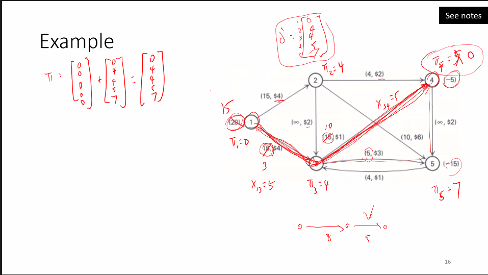
Minimum cost flow problem

when there is flow on a node, reduced cost is 0.

Successive Shortest Path Algorithm

Multicommodity flow problems

commodity's can be OD pairs like (1,3) signifying you want to move the commodity from node 1 to node 3.

Optimal conditions

1. shadow price of capacity constraint will equal 0, either the shadow price is greater than 0, ( binding ) or less than 0 non binding.
2. reduced cost always > 0 per commodity
3. reduced cost * flows = 0

Decomposition approach

when you remove a constraint you can only get better. We temporarily remove the capacity constraint. instead of having a hard capacity, we turn it into a contour, when you travel along the vector contour you get to find out how much penalty you get.

Possible ABQ Term project

Tram from Albuquerque to Santa fe

• evaluate alternatives

ART line

• evaluate an alternative

Homework 2

Resources

cost flow model cost flow model cost flow model cost flow model

Quiz 1

1 hour long, open book, online via Qualitrics survey.

10 randomized True/False questions, you need to respond with Justifications!

Materials covered

• Linear Programming
  • simplex algorithms
  • graphical method
  • shadow prices
  • reduced costs
  • dual problem
  • complementary slackness condition

Transportation problem

• transhipment/minimum cost flow problem
• shortest path problem
• Dijkstra algorithm
• successive shortest path algorithm
• multicommodity flow
• Lagrangian relaxation with subgradient optimization algorithm
• nonlinear programming traffic assignment problem

Learning Objectives

1. Multicommodity flow problem with decomposition algorithm
2. Adding congestion; decentralized decision making vs centralized decision making
3. User equilibrium versus system optimum
4. Beckmann's formulation, Karush Kuhn Tucker conditions link performance functions.

Readings

Chow Ch 3.1 - 3.2 Sheffi Ch 2.2-2.3,3

Lagrangian relaxation

Lemma: Legrangian bounding principle: for any vector w the value L(w) is a lower bound on the optimal objective function value Z.

1. solve for W
2. solve each OD's minimum cost flow with c' = c +w

Path-Based Formulation with Congestion

We can look at the problem as a nonlinear unncapacitated multicommodity flow model.

TIP

Use GRG nonlinear solver in excel

Centralized decision-making versus decentralized decisions.

when you can't make decisions as a whole - you have to make decisions based on

Marginal Cost + Average Cost

Coffee Shop Example

You go to coffee shop and are not sure how long it will take you to get through the line. The marginal cost is whether you are 1st, 2nd, 3rd etc in line, where the average cost is on avg how long does it take you.

Selfish Equilibrium reach by finding the minimum area under the average cost curves where they intersect for two parallel links with fixed demand. And movement past this point will incur additional cost

Wardrop's Principles ( 1952 )

Road Paper No. 36 at Road Engineering Division Meeting

No commuter can chose a different path and not be worse off, when equilibrium is reached.

1. The Journey times on all the routes actually used are equal and less than those which would be experienced by a single vehicle on any unused route. ( user equilibrium UE)
2. The average journey time is a minimum ( system optimum SO )

When there is no congestion effect, they are equal. Where marginal cost is equal to average cost.

Beckmann's UE Formulation | Traffic Assignment Problem ( Path based ) (TAP)

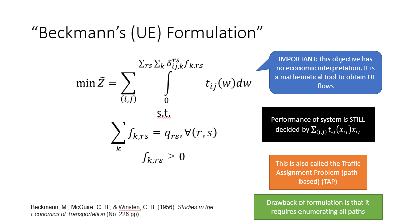
Beckmann M. McGuire & Winsten 1956 Studies in Economics of Transportation

WARNING

path flows are not unique!

What is unique?

You can't guarantee path flow, only link flow. Path decisions impact link flows, and link flows add up to path flows ( link path incidence matrix ).

• link cost
• link flow
• path cost

• objective needed to be consistent with decentralized behavior.
• measure in terms of path cost.
• There is no capacity.
• path costs need determine the observable link flows.

TIP

Path Flow problem, create a path-link incidence matrix. Put a 1 if the link is on the path.

WARNING

Performance is decided by iterating through every path

SO - integral of marginal cost UE - integral of average cost

Relating Link + Paths together

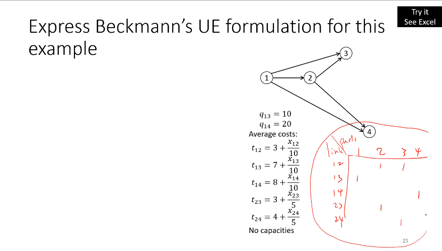
1. Integrate each average cost function by path
2. adding the sum of the integral of all the average costs

KKT Conditions

Karush-Kuhn-Tucker conditions

Sheffi 2.2 - 2.3

How we locate the solution in non-linear space.

TIP

Langrange multiplier ( shadow price of Non-linear problem )

Optimality conditions

1. flow * ( path cost - lagrange multiplier) for each path should equal 0
   1. either the flow will be 0 or the path - langrange multiplier = 0
2. path cost - langrange multiplier >= 0

Braess' Paradox

adding a link can make everyone worse off! ( but not always )

Line Planning Problem (LPP)

Borndörfer et al. (2007)

Line Planning Problem (LPP) - The problem is to design line routes and their frequencies in a street or track network such that a transportation volume, given by a so-called origin-destination matrix (OD-matrix), can be routed. There are two competing objectives minimize cost and decrease user discomfort. Discomfort can be measured as travel time and/or number of transfers/changes in mobility.

System Split - fixes the travel paths before the routes are known. Instead the model does not fix passenger paths according to a system split, but allows to freely route passengers according to the computed lines.

Model characteristics

Line Routes are simple bidirectional paths.

Transfers between lines are currently ignored in our model.

Frequencies indicate the (approximate) number of times vehicles need to be employed to serve the demand over the time horizon. However, as the frequencies mainly are used to adjust line capacities, we do (at present) not care so much about “nice” frequencies and view the fractional values as approximations or clues to “sensible” values.

NP Hard In computational complexity theory, NP-hardness (non-deterministic polynomial-time hardness) is the defining property of a class of problems that are informally "at least as hard as the hardest problems in NP". A simple example of an NP-hard problem is the subset sum problem. Stands for non-deterministic!

Computational Results

Potsdam Germany

We removed isolated nodes. Then, we iteratively removed “leaves” in the graph—i.e., nodes with only one neighbor—and iteratively contracted nodes with two neighbors. The preprocessed graph has 410 nodes, 106 of which were OD-nodes, and 891 edges

Conclusions

We proposed a new model for line planning in public transport that allows to generate lines dynamically and to freely route passengers according to the computed lines. The model allows to deal with manifold requirements from practice. We showed that LPs for a medium-sized town can be solved within reasonable quality with integer programming techniques. Our computational results indicate significant optimization potential. Our results on the polynomial time solvability of the LP relaxation for the case of logarithmic line lengths raises our hope that the model is suited to deal with larger problems as well.

Linear Programming

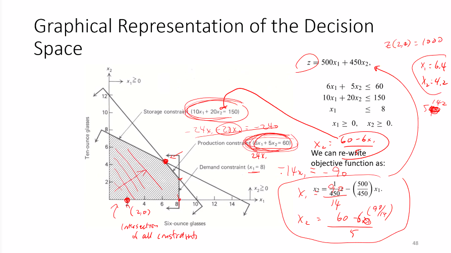
Linear programming is an optimization technique for a system of linear constraints and a linear objective function. An objective function defines the quantity to be optimized, and the goal of linear programming is to find the values of the variables that maximize or minimize the objective function.

Simplex Algorithm

Starts at a corner points of the feasible solution space and moves to the adjacent point which would improve the solution.

Gaussian Elimination

Moving one vertex to another by pivoting to isolate a different variable. We chose the variables to leave the basis by selecting the path of maximum increase to the objective function.

Canonical Form

1. all decision variables are constraint to be non-negative
2. All constraints, except non-negativity of decision variables are in the form of equality.
3. The RHS coefficients are all non-negative.
4. One decision variable is isolated in each constraint ( in the basis).

Transformation to canonical form examples

cx1 + cx2 + cx3 <= b

Add Slack variable

cx1 + cx2 + cx3 + s1 =  b

TIP

If the inequality is <= then + slack variable, otherwise if it is >= - the slack variable.

Example

z = 2x1  + x2 + x3

s.t.

2x1 + 3x2 - x3 <= 9
2x2 + x3 >= 4
x1 + x3 = 6

x1, x2 >= 0

Transform!

z - 2x1 - x2 - x3 = 0

s.t.

2x1 + 3x2 - x3 + s1 = 9
2x2 + x3 - s2 = 4
x1 + x3 = 6

x1, x2 >= 0

s1, s2 >= 0

WARNING

When setting up the tableau the stopping condition is when your objective variables are <= 0.

Deciding which column to pivot first. Select the column with the largest non zero objective value. From the selected column, you divide the b values by the respective column value. You select the smallest non negative value.

Perform row operations to isolate the given row/column value to make the given selected row all 0's except given value.

If the selected cell is the 2nd value, all other variables should be 0.

TIP

After solving the entire tableau all non isolated variables are non-basic.

0
1
0

Graphical Method

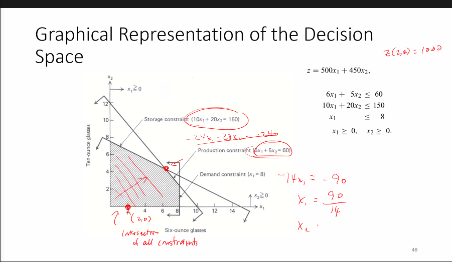
Create a graph of the linear constraints and see if they create a possible solution space.

TIP

A good way of testing is setting x and y equal to 0 and solving each constraint equation.

To find out which direction the inequality goes, test (0,0) and see if it is included in the given domain.

Shadow Price

How much one unit of each constraint resource is worth to us. When a constraint is non-binding, the shadow price should = 0. When is is binding, gives us the value of the constraint.

Reduced Cost

Type of shadow price to non-negativity constraint. If we have to produce one unit of a certain variable, how much would it cost to us.

Duel Problem

Complementary slackness condition

if shadow price is > 0, then the slack variable = 0. There can only be valuable to move the variable if it is binding. If the slack variable is > 0, then the shadow price = 0.

Check these conditions to see if the solution is optimal.

if you have reduced cost, moving one unit across the link - will add the given cost to your objective function.

Transportation Problem

Link-Path Incidence matrix

columns are paths and rows are link OD pairs.

WARNING

Transportation Problem Reduced Cost calculation if flow > 0 to calculate reduced cost = cost on link + shadow price - node potential = 0.

WARNING

Transhipment Reduced Cost

Transshipment/Minimum Cost Flow Problem

Send x units of flow from s to t as cheaply as possible.

Transportation Problem --> “bipartite graph” – all nodes are either sources or sinks; single commodity – demand from a sink node can be served by supply from any source node

Transshipment Problem or Minimum Cost Flow Problem --> nodes are either sources, sinks, or transshipment nodes; single commodity -- demand from a sink node can be served by supply from any source node Shortest path problem is a special case of this problem

Multicommodity Flow Problem --> nodes are either sources, sinks, or transshipment nodes; demand is defined per commodity (for passenger travel, each origin-destination (OD) pair is a commodity) When link costs are constant and there are no link capacities, this is the “All-or-Nothing” assignment in transportation planning models When link costs are functions of flow and there are no link capacities, this is the Traffic Assignment Problem

Shortest Path problem

The shortest path problem is about finding a path between 2 vertices in a graph such that the total sum of the edges weights is minimum.

Dijkstra Algorithm

label setting algorithm, where each iteration you close the shortest path. The closing condition is when you close your destination node.

Lagrangian Relaxation with Subgradient optimization

Multicommodity Flow Problem. We updated w (essentially the weight) each iteration to update the cost. If the w gets to 0, the node potential is negative.

::: w is non-negative :::

Traffic Assignment Problem

Uniqueness Theorem: The optimum of the formulation when the link cost functions are monotonically increasing with respect to the link flows, is unique with respect to the links flows.

We can only guarantee uniqueness of the links flows, but not the paths.

TIP

Nash equilibrium is a concept within game theory where the optimal outcome of a game is where there is no incentive to deviate from their initial strategy. ... Overall, an individual can receive no incremental benefit from changing actions, assuming other players remain constant in their strategies

Path Flow Uniqueness

Path decisions get you path flows. Then you get link flows by adding them up. You can get the path cost.

Karush-Kuhn-Tucker conditions ( see Sheffi 2.2 - 2.3)

In mathematical optimization, the Karush–Kuhn–Tucker (KKT) conditions, also known as the Kuhn–Tucker conditions, are first derivative tests (sometimes called first-order necessary conditions) for a solution in nonlinear programming to be optimal, provided that some regularity conditions are satisfied. wikipedia

TIP

a way to describe the location of the optimum to be at one of the constraints.

Langrange multiplier shadow price for NLPs. Must be greater than or equal to 0.

Frank-Wolfe Algorithm

excel example of LP

In excel Goal Seek for non linear programs

WARNING

objective is differentiable and convex!

nonlinear optimization algorithm, dimension matters! When there are vectors with thousands of dimensions, the iterative method does not work.

Multivariate unconstrained optimization review. Can be done iteratively via steepest descent based on using the gradient at your current location.

Gradient Descent

Gradient descent is a first-order iterative optimization algorithm for finding a local minimum of a differentiable function. To find a local minimum of a function using gradient descent, we take steps proportional to the negative of the gradient (or approximate gradient) of the function at the current point.

Instead of using gradient to draw line to simplify to 1-dimensional problem.

From the starting point x you find another point y corner point of the feasible decision space. Then draw a line between the two points x and y such that the function is f[ x + \alpha(y^n - x^n)]. The only unknown is \alpha to solve.

stopping condition(s), the decision variables don't change too much, or the objective function stops moving. Since the problem is convex you are moving towards an end goal so each iteration should be getting better.

TIP

Express assumes convex, each iteration should improve.

no path enumeration

algorithm is fast initially, then slow

Intermediate paths have no relation to actual final paths.

How to obtain SO ( system optimum )

• swap out avg cost t^/alpha for marginal cost m^/alpha

TIP

Convert Avg Cost to Marginal Cost

Multiply x and take first derivative.

Integer Programming

11/3/2020

Exercise

How to avoid NLP differentiation - successive averages

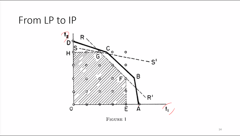
Integer programming - what happens when some or all the decisions variables are constrained to be discrete variables?

References

Sheffi Ch 12.2 BHM77 Ch 9.1 - 9.6 CHOW Ch 4.3.3

Why Integer Programming ( IP ) is more complex?

WARNING

Duality does not always apply to IP programs

Number of decision variables

For 8 node location problem, you end up with 72 decision variables.

Types of constraints

• pick one location, set binary variables to add up to 1
• pick at most 2 locations
• enforce at least one constraint

The Duel of the relaxed LP does not satisfy the strong duality condition. This is called Duality Gap.

Examples of constraint

Pick one location Set all your decision variables equal to 1. Force binary variables to add up to 1.

Pick at most 2 locations. Do that by setting inequality <=2.

Derivative-free method: Method of Successive Averages

set alpha to 1/n is guaranteed to converge for a convex objective function

Convergence, while guaranteed is very slow

instead of solving x + alpha * (y -x) = 0 for all the Sums, you instead use a static value 1/2, then 2/3, then 1/3 for the following iterations until you converge.

Stochastic user equilibrium - flow is a function of discrete choice-based route choice model for paths. There is probabilities for you to chose a given path.

Branch and Bound

You solve smaller linear programs each iteration. Each time your branch you are adding a constraint.

Reading

LO81 6.3 ( Larson and Odoni ) Chow 7.2.1 LO81 6.4 Chow 7.21-7.2.2

Minimum spanning tree ( MST ), Euler Tours

Type of optimization problem looking at how to connect a tree, to connect all the nodes together - in a least cost manner. Find a spanning tree that minimizes the costs of build.

TIP

Complete Graph - every node connected to every other node.

i.e.

How to connect every node ( neighborhood ) in a area together by a transit route.

$$ min Z = \sigma c\sup y y \sup y

s.t

$$

Prim's ( 1957 ) Algorithm

1. select any starting node. ( start of the tree )
2. select the node closest to any olf the nodes tree to join the tree.
3. Repeat Step 2 until all nodes have joined tree to create a spanning tree

WARNING

You find the closest one from the previous choice. You are not updating distances.

Euler Tour

That visits every link exactly once?

Called the Chinese Postman Problem

by Leonhard Euler in 18th century - the name was given after a 1962 paper in "Chinese Mathematics".

Euler's Theorem ( LO81 ch 6.4.2 )

The degree of a node in a connected graph is the number of links incident on the node.

Let an Euler tour be a circuit that traverses every edge on a graph exactly once. An Euler path is a path which traverses every edge on a graph exactly once.

A connected graph G possesses an Euler tour ( Euler path ) if and only if G contains exactly zero nodes of odd degree.

Travelling Salesman Problem

Connect all your nodes together with a tour ( only visit once ). Find the minimum distance route that begins at a given node of a network, visits all the members of a specified set of notes on the network at least once, and returns eventually to the initial node.

GeeksforGeeks

NP-HARD

Variant TSP Heuristics

WARNING

You don't know how good the solution is using this method.

Christofides' ( 1976 ) heuristic

1. find minimum spanning tree for the set of nodes call T
2. let $n0$ be the number of odd-degree nodes. Find minimum length match between these nodes. Let the graph of pairwise matches be M. Then let $H = M \upsilon T$
3. From Euler's Theorem, H should have an Eulerian tour. Draw this tour.
4. Apply triangle inequality to remove links traversed twice.

Method

1. Get Spanning tree
2. Find odd degree nodes
   1. find shortest connections between this subset of nodes.
3. Euler Tour
4. Triangle inequalities

TIP

Proved it would not be worst than 50% higher than the true minimized cost or 1.5x times worse than TST

$$ L(T) <= L(TST/link) < L(TST)

L(m) <= L(TST)/2

L(H) = L(m) + L(T) $$

Example

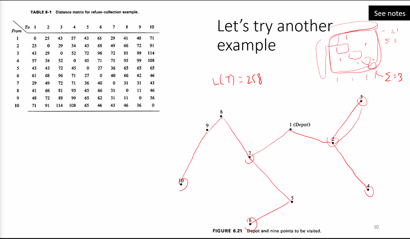
1. Create spanning Tree
2. create a minimal matching
3. Euler tour
4. remove triangles for improvements

Vehicle Routing Pick up + Drop off

1. vehicle visits one node, it has to visit the other node. one user with two nodes.
2. load can change during the course of the tour. The load can go up + down throughout the tour, by dropping off a consumer, increasing the available capacity.

Facility Location Problem

Given a graph undirected links, where to place a facility(s). it has to be on a node, or on a link. Depending on where we place the facility to assign demand nodes to optimize distance.

Might be locating them to minimize the average distance.

P-Medium Problem

(Hakimi 1964)

Average distance covered

Where do we want to place the facility, so that the average distance is minimized.

Hakimi's Theorem

The optimal solution will always lie on one of the nodes.

Consider an undirected network, with n nodes and m links where we seek k points.

distances are shortest paths.

Zone Assignment

Given a set of zones V connected by edges E, choose a subset of zones such that they are contiguous to a base zone 0. The total utility netted from all the served zones are maximized.

x^j = 1 if zone j is served, 0 otherwise.

q ^r is the demand served by zone j

y ^ij is a flow variable to link zones together ( to ensure contiguity )

Stackelberg Game ( leader-follower)

The leader can optimize, plugging in constraint of follower, the maximum product follower can create.

Two firm model, producing similar goods, where one firm sets prices first. Creating an inverse demand function.

Firm 1 the first mover, sets output and firm 2 observes output then sets own output. Firm 1, thinks about how firm 2 will respond to its initial output level - this is called firm 2 reaction function.

Bilvel problems are NP-hard and nonconvex.

Geometric probabilities ( continuous approximation model )

Stein D. M (1978) an asymptotic probabilistic analysis of a routing problem. Mathematics of Operations Research.

Approximate the length of tours, if they were to optimize tours.

Given a bounded region R with area a where n uniformally distributed nodes need to be visited --> length of shortest path through these points Ln has an asymptotic bound for some constraint b.